Today I will present the implementation of agglomerative hierarchical clustering in R. You can do a similar implementation in the language of your choice.

I will use the iris dataset here for explanation purpose. If you don’t have it in your R version you can download it from here

If you don’t have it in your R version you can download it from here. copy and save it to a text file called “iris.txt”. Please note, that there are no column headings to this dataset as of now. Now there are two ways to add the column headings.

Method 1: Open a new excel sheet and name the first row as sepalLength, sepalWidth, petalLength, petalWidth and after that you copy the dataset and paste it in excel sheet

Method 2: if you want to do it in R, you can use the function like colnames()

> colnames(iris)=c("sepalLength","sepalWidth","petalLeangth","petalWidth","Species") Now if you view the dataset like 

> View(iris) you would see that it has the column names rather than the default V1, V2, V3, V4,V5. On the R console if you type 
> summary(iris) you will see that it has 149 values in 5 variables of which the first four are numeric and the last variable Species is categorical.

Now, you can install the cluster package using

> install.packages(“cluster”) and after that load it using the library function like

>library(cluster)

I would recommend you to take a look at the cluster package so as to know how to implement the various clustering algorithms in it. To check that use

> ??cluster

I will now begin with the Agglomerative Clustering algorithm implementation in R first using the cluster package.

It is advisable to draw a random sample of data first otherwise the cluster dendogram will be messy because there are more than 100 values in 5 variables. To do this you can do like

my.dataframe[sample(nrow(dataset), size=), ] so for our example, the command will be

> iris.sample=iris[sample(nrow(iris),size=40),]

So now if you view the data like

> View(iris)

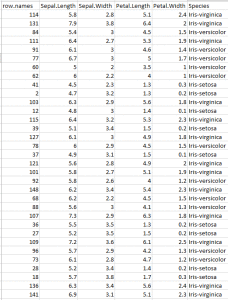
you will see that it’s randomly sampled. Notice the column row.names it lists random row numbers. This proves that the data is randomly sampled.

Now to apply agglomerative hierarchical clustering I will use the agnes function of the cluster package.

Let me first briefly describe the agnes function parameters here;

agnes(x, diss = inherits(x, “dist”), metric = “euclidean”, stand = FALSE, method = “average”, par.method,keep.diss = n < 100, keep.data = !diss, trace.lev = 0) 

where x= data frame or data matrix or the dissimilarity function.

In case of data matrix, all variables must be numeric. Missing Values (NA) are allowed. diss= logical flag if TRUE (which is the default value) then x is considered a dissimilarity matrix, if set FALSE then x is a matrix of observations by variable metric= euclidean distance or manhattan distance, stand= logical flag if TRUE (default value) then measurement in x are standardised before calculating the dissimilarity function. If x is already a dissimilarity matrix, then this argument will be ignored method= defines the clustering method to be used.

There are 6 types, “single”, “complete”, “average”,”ward”,”weighted”,”flexible” Now to apply the agglomerative hierarchical clustering, I will use the agnes function of the cluster package

> iris.hc=agnes(iris.sample, diss=FALSE, metric="euclidean", stand="TRUE", method="average")

Note: I have kept the diss=FALSE because iris.sample is a dataframe and not a dissimilarity matrix. I have chosen euclidean distance metric. And the clustering method is single link. You can try others.

Now to plot this dendogram use the plot function like

> plot(iris.hc)

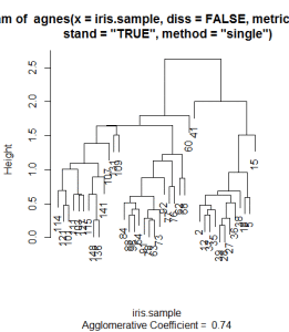
You will notice that the dendogram has row numbers of the random sample which is visually not very interpretive. At least for me this dendogram is not visually interpretive. So I will use the labels command in the plot function to show the names like

> plot(iris.hc, labels=iris.sample$Species)

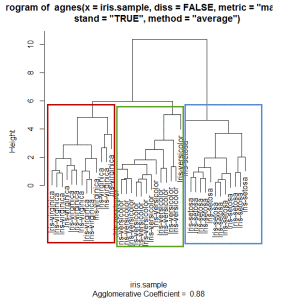
Clearly there are three clusters as shown in the plot.

Hope this helps.