1. Introduction
I serve as a reviewer to several ISI and Scopus indexed journals in Information Technology. Recently, I was reviewing an article, wherein the researchers had made a critical mistake in data analysis. They converted the original categorical data to continuous without providing a rigorous statistical treatment, nor, any justification to the loss of information if any. Thus, my motivation to develop this study, is borne out of their error.
We know the standard association measure between continuous variables is the product-moment correlation coefficient introduced by Karl Pearson. This measure determines the degree of linear association between continuous variables and is both normalized to lie between -1 and +1 and symmetric: the correlation between variables x and y is the same as that between y and x. the best-known association measure between two categorical variables is probably the chi-square measure, also introduced by Karl Pearson. Like the product-moment correlation coefficient, this association measure is symmetric, but it is not normalized. This lack of normalization provides one motivation for Cramer’s V, defined as the square root of a normalized chi-square value; the resulting association measure varies between 0 and 1 and is conveniently available via the assocstats function in the vcd package. An interesting alternative to Cramer’s V is Goodman and Kruskal’s tau, which is not nearly as well known and is asymmetric. This asymmetry arises because the tau measure is based on the fraction of variability in the categorical variable y that can be explained by the categorical variable x. 1
The data for this study is sourced from UCI Machine Learning repository. As it states in the data information section, “This data set includes descriptions of hypothetical samples corresponding to 23 species of gilled mushrooms in the Agaricus and Lepiota Family (pp. 500-525). Each species is identified as definitely edible, definitely poisonous, or of unknown edibility and not recommended. This latter class was combined with the poisonous one. The guide clearly states that there is no simple rule for determining the edibility of a mushroom;
Furthermore, the possible research questions, I want to explore are;
- Is significance test enough to justify a hypothesis?
- How to measure associations between categorical predictors?
2. Making data management decisions
As a first step, I imported the data in R environment as;
# Import data from UCI ML repo
> theURL<- "http://archive.ics.uci.edu/ml/machine-learning-databases/mushroom/agaricus-lepiota.data"
# Explicitly adding the column headers from the data dictionary
> mushroom.data<- read.csv(file = theURL, header = FALSE, sep = ",",strip.white = TRUE,
                     stringsAsFactors = TRUE,
                     col.names = c("class","cap-shape","cap-surface","cap-color","bruises",
                                   "odor","gill-attachment","gill-spacing","gill-size",
                                   "gill-color","stalk-shape","stalk-root","stalk-surface-above-ring",
                                   "stalk-surface-below-ring","stalk-color-above-ring","stalk-color-below-ring",
                                   "veil-type","veil-color","ring-number","ring-type","spore-print-color",
                                   "population","habitat"))
Next, I quickly summarize the dataset to get a brief glimpse. The reader’s should note that the data has no missing values. (Thanks to Junhewk Kim for pointing out the earlier error in data levels)
# Calculate number of levels for each variable
> mushroom.data.levels<-cbind.data.frame(Variable=names(mushroom.data), Total_Levels=sapply(mushroom.data,function(x){as.numeric(length(levels(x)))}))
> print(mushroom.data.levels)
                                     Variable Total_Levels
class                                       class            2
cap.shape                               cap.shape            6
cap.surface                           cap.surface            4
cap.color                               cap.color           10
bruises                                   bruises            2
odor                                         odor            9
gill.attachment                   gill.attachment            2
gill.spacing                         gill.spacing            2
gill.size                               gill.size            2
gill.color                             gill.color           12
stalk.shape                           stalk.shape            2
stalk.root                             stalk.root            5
stalk.surface.above.ring stalk.surface.above.ring            4
stalk.surface.below.ring stalk.surface.below.ring            4
stalk.color.above.ring     stalk.color.above.ring            9
stalk.color.below.ring     stalk.color.below.ring            9
veil.type                               veil.type            1
veil.color                             veil.color            4
ring.number                           ring.number            3
ring.type                               ring.type            5
spore.print.color               spore.print.color            9
population                             population            6
habitat                                   habitat            7
As we can see, the variable, gill.attachement has two levels (Thanks to Prof. Antony Unwin for pointing out the earlier error in gill.attachment). The variable, veil.type has one level.
The different levels are uninterpretable in their current format. I will use the data dictionary and recode the levels into meaningful names.
> levels(mushroom.data$class)<- c("edible","poisonous")
> levels(mushroom.data$cap.shape)<-c("bell","conical","flat","knobbed","sunken","convex")
> levels(mushroom.data$cap.surface)<- c("fibrous","grooves","smooth","scaly")
> levels(mushroom.data$cap.color)<- c("buff","cinnamon","red","gray","brown","pink","green","purple","white","yellow")
> levels(mushroom.data$bruises)<- c("bruisesno","bruisesyes")
> levels(mushroom.data$odor)<-c("almond","creosote","foul","anise","musty","nosmell","pungent","spicy","fishy")
> levels(mushroom.data$gill.attachment)<- c("attached","free")
> levels(mushroom.data$gill.spacing)<- c("close","crowded")
> levels(mushroom.data$gill.size)<-c("broad","narrow")
> levels(mushroom.data$gill.color)<- c("buff","red","gray","chocolate","black","brown","orange","pink","green","purple","white","yellow")
> levels(mushroom.data$stalk.shape)<- c("enlarging","tapering")
> table(mushroom.data$stalk.root) # has a missing level coded as ?
   	?    b    c    e    r
2480 3776  556 1120  192
> levels(mushroom.data$stalk.root)<- c("missing","bulbous","club","equal","rooted")
> levels(mushroom.data$stalk.surface.above.ring)<-c("fibrous","silky","smooth","scaly")
> levels(mushroom.data$stalk.surface.below.ring)<-c("fibrous","silky","smooth","scaly")
> levels(mushroom.data$stalk.color.above.ring)<- c("buff","cinnamon","red","gray","brown",                "orange","pink","white","yellow")
> levels(mushroom.data$stalk.color.below.ring)<- c("buff","cinnamon","red","gray","brown",      "orange","pink","white","yellow")
> levels(mushroom.data$veil.type)<-c("partial")
> levels(mushroom.data$veil.color)<- c("brown","orange","white","yellow")
> levels(mushroom.data$ring.number)<-c("none","one","two")
> levels(mushroom.data$ring.type)<- c("evanescent","flaring","large","none","pendant")
> levels(mushroom.data$spore.print.color)<- c("buff","chocolate","black","brown","orange","green","purple","white","yellow")
> levels(mushroom.data$population)<- c("abundant","clustered","numerous","scattered","several","solitary")
> levels(mushroom.data$habitat)<-c("woods","grasses","leaves","meadows","paths","urban","waste")
3. Initial data visualization
Since, we are dealing with categorical data, plotting it is slightly different. Here we use bar charts/plots or mosaic plots rather than dot plots or scatter plots. (Thanks to Prof. Antony Unwin for pointing it out). The dot plot is useful for plotting continuous variables. It can be used, to plot categorical variables, but then such a visualization will be confusing.
a. Univariate data visualization (Stacked Bar plot)
> p<- ggplot(data = mushroom.data)
> p+geom_bar(mapping = aes(x = cap.shape, fill=class), position = position_dodge())+ theme(legend.position = "top")
> table(mushroom.data$cap.shape, mushroom.data$class)
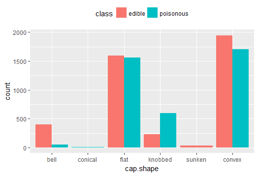
Fig-1: Mushroom cap-shape and class
From Fig-1, we can easily notice, the mushrooms with a, flat cap-shape are mostly edible (n=1596) and an equally similar number are poisonous (n=1556). A majority of bellshaped mushrooms (n=404) are edible. All conical cap-shaped mushrooms are poisonous (n=4). And, all sunken cap-shaped mushrooms are edible (n=32).
b. How is habitat related to class? (Mosaic Plot)
> library(vcd) # for mosaicplot()
> table(mushroom.data$habitat, mushroom.data$class) # creates a contingency table

          edible poisonous
  	woods     1880      1268
  	grasses   1408       740
  	leaves     240       592
  	meadows    256        36
  	paths      136      1008
  	urban       96       272
  	waste      192         0
> mosaicplot(~ habitat+class, data = mushroom.data,cex.axis = 0.9, shade = TRUE,
       main="Bivariate data visualization",
       sub = "Relationship between mushroom habitat and class",
       las=2, off=10,border="chocolate",xlab="habitat", ylab="class" )
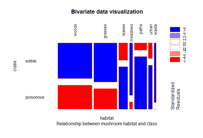
Fig-2: Mushroom habitat and class
From Fig-2, we see a majority of mushrooms that live in woods, grasses, leaves, meadows and paths are edible. Surprisingly, the one’s living in waste areas are entirely edible.
c. How is population related with class?
> table(mushroom.data$population, mushroom.data$class)

        edible poisonous
  abundant     384         0
  clustered    288        52
  numerous     400         0
  scattered    880       368
  several     1192      2848
  solitary    1064       648

> mosaicplot(~ population+class, data = mushroom.data,
       cex.axis = 0.9, shade = TRUE,
       main="Bivariate data visualization",
       sub = "Relationship between mushroom population and class",
       las=2, off=10,border="chocolate",xlab="population", ylab="class")
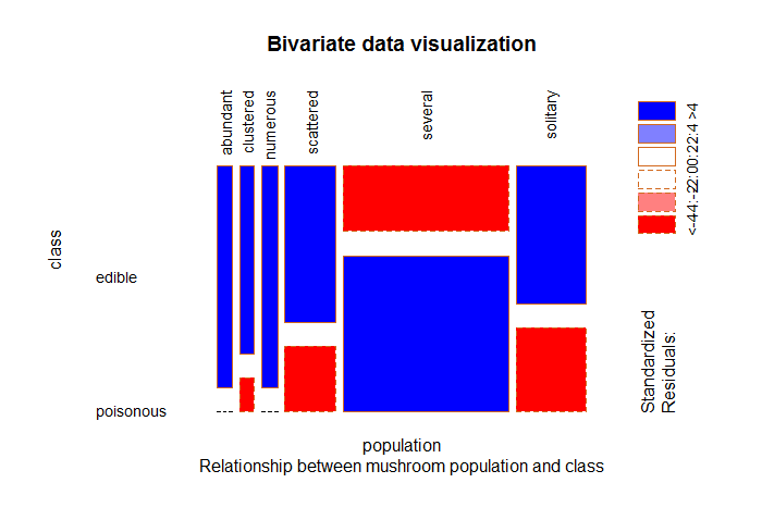
Fig-3: Mushroom population and class
From Fig-3, we can see a majority of mushroom population that is either, clustered, scattered, several or solitary are edible. The mushrooms that are either abundant or numerous in population are completely edible.
Although, there could be many other pretty visualizations but I will leave that as a future work.
I will now focus on exploratory data analysis.
4. Exploratory data analysis
a. Correlation detection & treatment for categorical predictors
If we look at the structure of the dataset, we notice that each variable has several factor levels. Moreover, these levels are unordered. Such unordered categorical variables are termed as nominal variables. The opposite of unordered is ordered, we all know that. The ordered categorical variables are called, ordinal variables.
“In the measurement hierarchy, interval variables are highest, ordinal variables are next, and nominal variables are lowest. Statistical methods for variables of one type can also be used with variables at higher levels but not at lower levels.”, see the book, Categorical Data Analysis by Alan Agresti
I found this cheat-sheet that can aid in determining the right kind of test to perform on categorical predictors (independent/explanatory variables). Also, this SO post is very helpful. See the answer by user gung.
For categorical variables, the concept of correlation can be understood in terms of significance test and effect size (strength of association)
The Pearson’s chi-squared test of independence is one of the most basic and common hypothesis tests in the statistical analysis of categorical data. It is a significance test. Given two categorical random variables, X and Y, the chi-squared test of independence determines whether or not there exists a statistical dependence between them. Formally, it is a hypothesis test. The chi-squared test assumes a null hypothesis and an alternate hypothesis. The general practice is, if the p-value that comes out in the result is less than a pre-determined significance level, which is 0.05 usually, then we reject the null hypothesis.
H0: The The two variables are independent
H1: The The two variables are dependent
The null hypothesis of the chi-squared test is that the two variables are independent and the alternate hypothesis is that they are related.
To establish that two categorical variables (or predictors) are dependent, the chi-squared statistic must have a certain cutoff. This cutoff increases as the number of classes within the variable (or predictor) increases.
In section 3a, 3b and 3c, I detected possible indications of dependency between variables by visualizing the predictors of interest. In this section, I will test to prove how well those dependencies are associated. First, I will apply the chi-squared test of independence to measure if the dependency is significant or not. Thereafter, I will apply the Goodman’s Kruskal Tau test to check for effect size (strength of association).
i. Pearson’s chi-squared test of independence (significance test)
> chisq.test(mushroom.data$cap.shape, mushroom.data$cap.surface, correct = FALSE)

Pearson's Chi-squared test

data:  mushroom.data$cap.shape and mushroom.data$cap.surface
X-squared = 1011.5, df = 15, p-value < 2.2e-16
since the p-value is < 2.2e-16 is less than the cut-off value of 0.05, we can reject the null hypothesis in favor of alternative hypothesis and conclude, that the variables, cap.shape and cap.surface are dependent to each other.
> chisq.test(mushroom.data$habitat, mushroom.data$odor, correct = FALSE)

Pearson's Chi-squared test

data:  mushroom.data$habitat and mushroom.data$odor
X-squared = 6675.1, df = 48, p-value < 2.2e-16
Similarly, the variables habitat and odor are dependent to each other as the p-value < 2.2e-16 is less than the cut-off value 0.05.
ii. Effect size (strength of association)
The measure of association does not indicate causality, but association–that is, whether a variable is associated with another variable. This measure of association also indicates the strength of the relationship, whether, weak or strong.
Since, I’m dealing with nominal categorical predictor’s, the Goodman and Kruskal’s tau measure is appropriate. Interested readers are invited to see pages 68 and 69 of the Agresti book. More information on this test can be seen here
> library(GoodmanKruskal)
> varset1<- c("cap.shape","cap.surface","habitat","odor","class")
> mushroomFrame1<- subset(mushroom.data, select = varset1)
> GKmatrix1<- GKtauDataframe(mushroomFrame1)
> plot(GKmatrix1, corrColors = "blue")
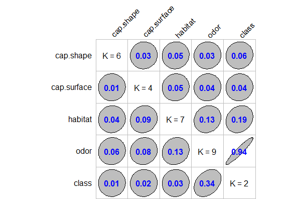
In Fig-4, I have shown the association plot. This plot is based on the corrplot library. In this plot the diagonal element K refers to number of unique levels for each variable. The off-diagonal elements contain the forward and backward tau measures for each variable pair. Specifically, the numerical values appearing in each row represent the association measure τ(x,y)τ(x,y) from the variable xx indicated in the row name to the variable yy indicated in the column name.
The most obvious feature from this plot is the fact that the variable odor is almost perfectly predictable (i.e. τ(x,y)=0.94) from class and this forward association is quite strong. The forward association suggest that x=odor (which has levels “almond”, “creosote”, “foul”, “anise”, “musty”, “nosmell”, “pungent”, “spicy”, “fishy”) is highly predictive of y=class (which has levels “edible”, “poisonous”). This association between odor and class is strong and indicates that if we know a mushroom’s odor than we can easily predict its class being edible or poisonous.
On the contrary, the reverse association y=class and x=odor(i.e. τ(y,x)=0.34; is a strong association and indicates that if we know the mushroom’s class being edible or poisonous than its easy to predict its odor.
Earlier we have found cap.shape and cap.surface are dependent to each other (chi-squared significance test). Now, let’s see if the association is strong too or not. Again, from Fig-4, both the forward and reverse association suggest that x=cap shape is weakly associated to y=cap surface (i.e.τ(x,y)=0.03) and (i.e.τ(y,x)=0.01). Thus, we can safely say that although these two variables are significant but they are association is weak; i.e. it will be difficult to predict one from another.
Similarly, many more associations can be interpreted from plot-4. I invite interested reader’s to explore it further.
5. Conclusion
The primary objective of this study was to drive the message, do not tamper the data without providing a credible justification. The reason I chose categorical data for this study to provide an in-depth treatment of the various measures that can be applied to it. From my prior readings of statistical texts, I could recall that significance test alone was not enough justification; there had to be something more. It is then, I found about the different types of association measures, and it sure did clear my doubts. In my next post, I will continue the current work by providing inferential and predictive analysis. For interested reader’s, I have uploaded the complete code on my Github repository in here
comments powered by Disqus