Introduction
While reading the local daily, “The Star”, my attention was caught by headlines discussing an ongoing political or social discussion on the country’s financial state. Often, it is interesting to know the underlying cause of a certain political debate or the factors contributing to an increase or decrease in inflation. “A large income is the best recipe for happiness I ever heard of” quotes the famous English novelist Jane Austen. Income is a primary concern that dictates the standard of living and economic status of an individual. Taking into account, its importance and impact on determining a nation’s growth, this study aims at presenting meaningful insights which can be used to serve as the basis for many wiser decisions that could be taken by the nation’s administrators.
This study is organized as follows;
-
Research question
-
The dataset
-
Making data management decisions
A. Exploratory Data Analysis (EDA)
- Data preprocessing (collapse the factor levels & re-coding)
- Missing data visualization
- Some obvious relationships
- Some not-so-obvious relationships
B. Correlation Detection & Treatment
- Detecting skewed variables
- Skewed variables treatment
- Correlation detection
-
Predictive data analytics
- Creating the train and test dataset
- Fit a Logistic Regression Model
- Fit a Decision Tree Model
- Fit a Support Vector Machine (SVM) classification model
- Fit a Random Forest (RF) classification model
-
Conclusion
1. Research question
This study is driven by the question, “Predict if a person’s income is above or below 50K$/yr given certain features(both quantitative and qualitative)..”
2. The dataset
The dataset used for the analysis is an extraction from the 1994 census data by Barry Becker and donated to the UCI Machine Learning repository. This dataset is popularly called the “Adult” data set.
3. Making data management decisions
With the research question in place and the data source identified, we begin the data storytelling journey. But wait, we first require to load the data,
# Import the data from a url
> theUrl<-"http://archive.ics.uci.edu/ml/machine-learning-databases/adult/adult.data"
> adult.data<- read.table(file = theUrl, header = FALSE, sep = ",",
                    strip.white = TRUE, stringsAsFactors = TRUE,
                    col.names=c("age","workclass","fnlwgt","education","educationnum","maritalstatus",                      "occupation","relationship","race","sex","capitalgain","capitalloss",                     "hoursperweek","nativecountry","income")
                    )
> dim (adult.data)
> [1] 32561    15
A. Exploratory Data Analysis (EDA)
The function, col.names() adds the user-supplied column names to the dataset. We also see 32,561 observations in 15 variables. As always, we look at the data structure,
Immediately, a few problems can be spotted. First, there are some categorical variables where the missing levels are coded as ?; Second, there are more than 10 levels for some categorical variables.
- Data preprocessing (collapse the factor levels & re-coding)
We begin by collapsing the factor levels to meaningful and relevant levels. We have also re-coded the missing levels denoted in the original data as ? to misLevel.
> levels(adult.data$workclass)<- c("misLevel","FedGov","LocGov","NeverWorked","Private","SelfEmpNotInc","SelfEmpInc","StateGov","NoPay")

> levels(adult.data$education)<- list(presch=c("Preschool"), primary=c("1st-4th","5th-6th"),upperprim=c("7th-8th"), highsch=c("9th","Assoc-acdm","Assoc-voc","10th"),secndrysch=c("11th","12th"), graduate=c("Bachelors","Some-college"),master=c("Masters"), phd=c("Doctorate"))

> levels(adult.data$maritalstatus)<- list(divorce=c("Divorced","Separated"),married=c("Married-AF-	spouse","Married-civ-spouse","Married-spouse-absent"),notmarried=c("Never-married"),widowed=c("Widowed"))

> levels(adult.data$occupation)<- list(misLevel=c("?"), clerical=c("Adm-clerical"), lowskillabr=c("Craft-repair","Handlers-cleaners","Machine-op-inspct","Other-service","Priv-house-	serv","Prof-specialty","Protective-serv"),highskillabr=c("Sales","Tech-support","Transport-moving","Armed-Forces"),agricultr=c("Farming-fishing"))

> levels(adult.data$relationship)<- list(husband=c("Husband"), wife=c("Wife"), outofamily=c("Not-in-family"),unmarried=c("Unmarried"), relative=c("Other-relative"), ownchild=c("Own-child"))

levels(adult.data$nativecountry)<- list(misLevel=c("?","South"),SEAsia=c("Vietnam","Laos","Cambodia","Thailand"),Asia=c("China","India","HongKong","Iran","Philippines","Taiwan"),NorthAmerica=c("Canada","Cuba","Dominican-Republic","Guatemala","Haiti","Honduras","Jamaica","Mexico","Nicaragua","Puerto-Rico","El-Salvador","United-States"), SouthAmerica=c("Ecuador","Peru","Columbia","Trinadad&Tobago"),Europe=c("France","Germany","Greece","Holand-Netherlands","Italy","Hungary","Ireland","Poland","Portugal","Scotland","England","Yugoslavia"),PacificIslands=c("Japan","France"),Oceania=c("Outlying-US(Guam-USVI-etc)"))
Now, here is an interesting finding about this dataset. Although, the response (dependent) variable can be considered as binary but there are majority of predictors (independent) that are categorical with many levels.
According to Agresti [1], “Categorical variables have two primary types of scales. Variables having categories without a natural ordering are called nominal. Example, mode of transportation to work (automobile, bicycle, bus, subway, walk). For nominal variables, the order of listing the categories is irrelevant. The statistical analysis does not depend on that ordering. Many categorical variables do have ordered categories. Such variables are called ordinal. Examples are size of automobile (subcompact, compact, midsize, large). Ordinal variables have ordered categories, but distances between categories are unknown. Although a person categorized as moderate is more liberal than a person categorized as conservative, no numerical value describes how much more liberal that person is. An interval variable is one that does have numerical distances between any two values.”
“A variable’s measurement scale determines which statistical methods are appropriate. In the measurement hierarchy, interval variables are highest, ordinal variables are next, and nominal variables are lowest. Statistical methods for variables of one type can also be used with variables at higher levels but not at lower levels. For instance, statistical methods for nominal variables can be used with ordinal variables by ignoring the ordering of categories. Methods for ordinal variables cannot, however, be used with nominal variables, since their categories have no meaningful ordering.”
“Nominal variables are qualitative, distinct categories differ in quality, not in quantity. Interval variables are quantitative, distinct levels have differing amounts of the characteristic of interest.”
Therefore, we can say that all the categorical predictors in this study are nominal in nature. Also note that R will implicitly coerce the categorical variable with levels into numerical values so there is no need to explicitly do the coercion.
we check the data structure again and notice that predictors, education,occupation and native.country have 11077, 4066 and 20 missing value respectively. We show this distribution in Fig-1.
aggr_plot <- aggr(adult.data, col=c('navyblue','red'), numbers=TRUE, sortVars=TRUE,
              labels=names(adult.data), cex.axis=.7, gap=3,
              ylab=c("Histogram of missing data","Pattern")
              )
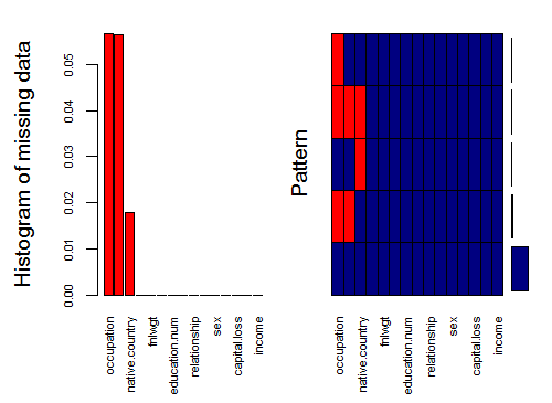
Fig-1: Missing Data Visualization
Now, some scholars suggest that missing data imputation for categorical variables introduce bias in the data while others oppose it. From, an analytical perspective we will impute the missing data and will use the missForest library. The reason why we are imputing is because some classification algorithms will fail if they are passed with data containing missing values.
# Missing data treatment
> library(missForest)
> imputdata<- missForest(adult.data)
# check imputed values
> imputdata$ximp
# assign imputed values to a data frame
> adult.cmplt<- imputdata$ximp
- Some obvious relationships
A majority of the working adults are between 25 to 65 years of age. From Fig-2, we see that adults below 30 years earn <=50k a year while those above 43 years of age earn greater than fifty thousand dollars. This leads to the assumption that experience surely matters to earn more.
> boxplot (age ~ income, data = adult.cmplt,
     main = "Age distribution for different income levels",
     xlab = "Income Levels", ylab = "Age", col = "salmon")
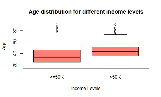
Fig-2: Boxplot for age and income
Evidently, those who invest more time at workplace tend to be earning more as depicted by Fig-3.
It is also interesting to note in Fig-5, that there are roughly 10% of people with doctorate degrees working in low-skilled jobs and earning greater than 50k/year.
> boxplot (hoursperweek ~ income, data = adult.cmplt,
     main = "More work hours, more income",
     xlab = "Income Levels", ylab = "Hours per week", col = "salmon")
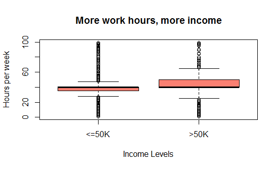
Fig-3: Boxplot for hours per week in office and income
- Some not-so-obvious relationships
Question: Does higher skill-set (sales, technical-support, transport movers, armed forces) is a guarantor to high income?
Answer: We explore this question by plotting occupation against income levels. As shown in Fig-4, its evident that acquiring a high skill set does not guarantee increased income. The workers with a low skill set (craft-repair, maintenance services, cleaner, private house security) earn more as compared to those with higher skill set.
> qplot(income, data = adult.cmplt, fill = occupation) + facet_grid (. ~ occupation)
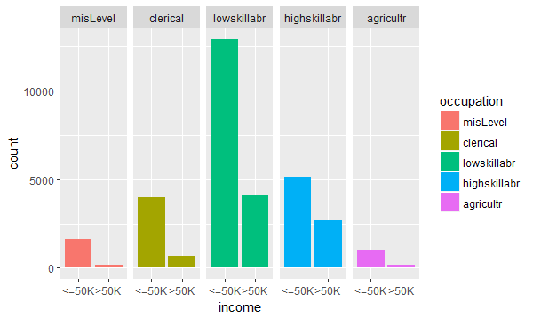
Fig-4: Q-plot for occupation and income
Question: Does higher education help earn more money?
Answer: We explore this question by plotting education against income levels. As shown in Fig-5
> qplot(income, data = adult.cmplt, fill = education) + facet_grid (. ~ education)
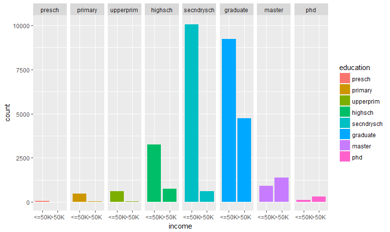
Fig-5: Q-plot for education and income
From Fig-5, we can easily make out that the number of graduates earning >50K are more than the high school or upper-primary school educated. However, we also notice that they are certainly higher in number when compared to master’s or phd degree holders. It makes sense because if for example, in a given academic session, there will be say 90% graduates, 30% masters, <10% phd degree holders. It is also unfortunate to know that there are roughly 10% of people (n=94) with doctorate degrees working in low-skilled jobs and earning less than 50k/year!
We further drill down in this low income group bracket, shown in Fig-5, we realize that majority of them are white male married workers closely followed by the blacks and the Asia-Pacific islanders.
> qplot(income, data = adult.cmplt, fill = relationship) + facet_grid (. ~ race)
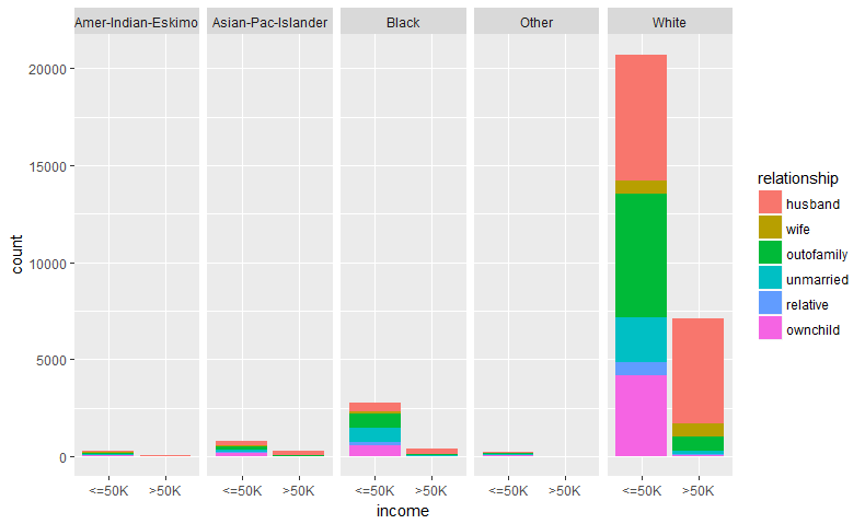
Fig-5: Q-plot for race, relationship and income
- Detecting skewed variables
A variable is considered, highly skewed if its absolute value is greater than 1. A variable is considered, moderately skewed if its absolute value is greater than 0.5.
> skewedVars<- NA
> library(moments) # for skewness()
> for(i in names(adult.cmplt)){
...   if(is.numeric(adult.cmplt[,i])){
...     if(i != "income"){
...       # Enters this block if variable is non-categorical
...       skewVal <- skewness(adult.cmplt[,i])
...       print(paste(i, skewVal, sep = ": "))
...       if(abs(skewVal) > 0.5){
...         skewedVars <- c(skewedVars, i)
...       }
...     }
...   }
... }
[1] "fnlwgt: 1.44691343514233"
[1] "capitalgain: 11.9532969981943"
[1] "capitalloss: 4.59441745643977"
[1] "age: 0.558717629239857"
[1] "educationnum: -0.311661509635468"
[1] "hoursperweek: 0.227632049774777"
We find that the predictors, fnlwgt,capitalgain and capitalloss are highly skewed as their absolute value is greater than 0.5.
- Skewed variable treatment
Post identifying the skewed variables, we proceed to treating them by taking the log transformation. But, first we rearrange/reorder the columns for simplicity;
> adult.cmplt<- adult.cmplt[c(3,11:12,1,5,13,2,4,6:10,14:15)]
> str(adult.cmplt)
'data.frame':	32561 obs. of  15 variables:
 $ fnlwgt       : num  77516 83311 215646 234721 338409 ...
 $ capitalgain  : num  2174 0 0 0 0 ...
 $ capitalloss  : num  0 0 0 0 0 0 0 0 0 0 ...
 $ age          : num  39 50 38 53 28 37 49 52 31 42 ...
 $ educationnum : num  13 13 9 7 13 14 5 9 14 13 ...
 $ hoursperweek : num  40 13 40 40 40 40 16 45 50 40 ...
 $ workclass    : Factor w/ 9 levels "misLevel","FedGov",..: 8 7 5 5 5 5 5 7 5 5 ...
 $ education    : Factor w/ 8 levels "presch","primary",..: 6 6 5 5 6 7 4 6 7 6 ...
 $ maritalstatus: Factor w/ 4 levels "divorce","married",..: 3 2 1 2 2 2 2 2 3 2 ...
 $ occupation   : Factor w/ 5 levels "misLevel","clerical",..: 2 5 3 3 3 3 3 4 3 4 ...
 $ relationship : Factor w/ 6 levels "husband","wife",..: 3 1 3 1 2 2 3 1 3 1 ...
 $ race         : Factor w/ 5 levels "Amer-Indian-Eskimo",..: 5 5 5 3 3 5 3 5 5 5 ...
 $ sex          : Factor w/ 2 levels "Female","Male": 2 2 2 2 1 1 1 2 1 2 ...
 $ nativecountry: Factor w/ 8 levels "misLevel","SEAsia",..: 4 4 4 4 4 4 4 4 4 4 ...
 $ income       : Factor w/ 2 levels "<=50K",">50K": 1 1 1 1 1 1 1 2 2 2 ...
We took a log transformation. Post skewed treatment, we notice that capitalgain & capitalloss have infinite values so we removed them from subsequent analysis.
> adult.cmplt.norm<- adult.cmplt
> adult.cmplt.norm[,1:3]<- log(adult.cmplt[1:3],2) # where 2 is log base 2
> adult.cmplt.norm$capitalgain<- NULL
> adult.cmplt.norm$capitalloss<-NULL
- Correlation detection
We now checked for variables with high correlations to each other. Correlation measures the relationship between two variables. When two variables are so highly correlated that they explain each other (to the point that one can predict the variable with the other), then we have collinearity (or multicollinearity) problem. Therefore, its is important to treat collinearity problem. Let us now check, if our data has this problem or not.
Again, it is important to note that correlation works only for continuous variables. We can calculate the correlations by using the cor() as shown;
> correlat<- cor(adult.cmplt.norm[c(1:4)])
> corrplot(correlat, method = "pie")
> highlyCor <- colnames(adult.cmplt.num)[findCorrelation(correlat, cutoff = 0.7, verbose = TRUE)]
All correlations <= 0.7
> highlyCor # No high Correlations found
character(0)
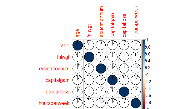
Fig-7: Correlation detection
From Fig-7, its evident that none of the predictors are highly correlated to each other. We now proceed to building the prediction model.
###4. Predictive data analytics
In this section, we will discuss various approaches applied to model building, predictive power and their trade-offs.
A. Creating the train and test dataset
We now divide the data into 75% training set and 25% testing set. We also created a root mean square evaluation function for model testing.
> ratio = sample(1:nrow(adult.cmplt), size = 0.25*nrow(adult.cmplt))
> test.data = adult.cmplt[ratio,] #Test dataset 25% of total
> train.data = adult.cmplt[-ratio,] #Train dataset 75% of total
> dim(train.data)
[1] 24421    15
> dim(test.data)
[1] 8140   15
**B. Fit a Logistic Regression Model **
We fit a logistic regression model.
> glm.fit<- glm(income~., family=binomial(link='logit'),data = train.data)
Warning message:
glm.fit: fitted probabilities numerically 0 or 1 occurred
This Warning: glm.fit: fitted probabilities numerically 0 or 1 occurred means that the data is possibly linearly separable. Let’s look at the summary for the model.
> summary(glm.fit)
Call:
glm(formula = income ~ ., family = binomial(link = "logit"),
data = train.data)

Deviance Residuals:
Min       1Q   Median       3Q      Max
-5.2316  -0.4639  -0.1713  -0.0311   3.4484

Coefficients: (1 not defined because of singularities)
                              Estimate     Std. Error z value Pr(>|z|)
(Intercept)                 -27.1523662282 171.0342617549  -0.159 0.873863
age                           0.0274845471   0.0019376261  14.185  < 2e-16 ***
workclassFedGov               0.4073987950   0.2085465221   1.954 0.050759 .
workclassLocGov              -0.3070912295   0.1944447001  -1.579 0.114262
workclassNeverWorked        -10.5345275621 510.1141392772  -0.021 0.983524
workclassPrivate             -0.1374981405   0.1816628614  -0.757 0.449118
workclassSelfEmpNotInc       -0.1132407363   0.1995129601  -0.568 0.570316
workclassSelfEmpInc          -0.6270437314   0.1773500692  -3.536 0.000407 ***
workclassStateGov            -0.4387629630   0.2049449847  -2.141 0.032284 *
workclassNoPay              -13.9146466535 367.0432320049  -0.038 0.969759
fnlwgt                        0.0000004226   0.0000002029   2.083 0.037252 *
educationprimary             18.6369757615 171.0337793366   0.109 0.913229
educationupperprim           18.6015984474 171.0337199499   0.109 0.913393
educationhighsch             19.4272321191 171.0336543439   0.114 0.909565
educationsecndrysch          18.3381423049 171.0336420490   0.107 0.914615
educationgraduate            20.1855955674 171.0336647250   0.118 0.906051
educationmaster              20.6169432260 171.0337212540   0.121 0.904053
educationphd                 20.8122445845 171.0338205358   0.122 0.903149
educationnum                  0.1301601416   0.0134594027   9.671  < 2e-16 ***
maritalstatusmarried          0.6518153342   0.1922871329   3.390 0.000699 ***
 [ reached getOption("max.print") -- omitted 26 rows ]
---
Signif. codes:  0 ‘***’ 0.001 ‘**’ 0.01 ‘*’ 0.05 ‘.’ 0.1 ‘ ’ 1

(Dispersion parameter for binomial family taken to be 1)

Null deviance: 26907  on 24420  degrees of freedom
Residual deviance: 14892  on 24376  degrees of freedom
AIC: 14982

Number of Fisher Scoring iterations: 14
Its evident that the significant predictors are age, workclassSelfEmpInc,fnlwgt,educationnum and maritalstatusmarried. As for the statistical significant variables, age and educationnum has the lowest p value suggesting a strong association with the response, income.
The null deviance shows how well the response is predicted by the model with nothing but an intercept. Deviance is a measure of goodness of fit of a generalized linear model. it’s a measure of badness of fit–higher numbers indicate worse fit. The residual deviance shows how well the response is predicted by the model when the predictors are included. From your example, it can be seen that the residual deviance decreases by 12115 (27001-14886) when 15 predictors were added to it.(note: degrees of freedom = no. of observations – no. of predictors). This decrease in deviance is evidence of significant fit. If the deviance would have increased it would indicate a significant lack of fit. The AIC is 14976. The Akaike Information Criterion (AIC) provides a method for assessing the quality of your model through comparison of related models. It’s based on the Deviance, but penalizes you for making the model more complicated. Much like adjusted R-squared, it’s intent is to prevent you from including irrelevant predictors. However, unlike adjusted R-squared, the number itself is not meaningful. If you have more than one similar candidate models (where all of the variables of the simpler model occur in the more complex models), then you should select the model that has the smallest AIC. So AIC is useful for comparing models, but isn’t interpretable on its own.
We now create another logistic model that includes only the significant predictors.
> glm.fit1<- glm(income ~ age + workclass + educationnum + fnlwgt + maritalstatus, family=binomial(link='logit'),data = train.data)
Now we can run the anova() function on the improved model to analyze the table of deviance.
> anova(glm.fit, glm.fit1, test="Chisq")

Analysis of Deviance Table

Model 1: income ~ age + workclass + fnlwgt + education + educationnum +
maritalstatus + occupation + relationship + race + sex +
capitalgain + capitalloss + hoursperweek + nativecountry
Model 2: income ~ age + workclass + educationnum + fnlwgt + maritalstatus
  	Resid. Df Resid. Dev  Df Deviance  Pr(>Chi)
1     24376      14892
2     24406      18428 -30  -3536.1 < 2.2e-16 ***
---
Signif. codes:  0 ‘***’ 0.001 ‘**’ 0.01 ‘*’ 0.05 ‘.’ 0.1 ‘ ’ 1
By conducting the anova test, it performs the Chi-square test to compare glm.fit and glm.fit1 (i.e. it tests whether reduction in the residual sum of squares are statistically significant or not). The test shows that, Model 2 is statistically significant as the p value is less than 0.05. Therefore, the predictors, (age + workclass + educationnum + fnlwgt + maritalstatus) are relevant for the model. See this links for details, 1, 2 and 3.
We now test the logistic model on all predictors and make predictions on unseen data.
> set.seed(1234)
> glm.pred<- predict(glm.fit, test.data, type = "response")
> hist(glm.pred, breaks=20)
> hist(glm.pred[test.data$income], col="red", breaks=20, add=TRUE)
> table(actual= test.data$income, predicted= glm.pred>0.5)
   predicted
actual  FALSE TRUE
  	<=50K  5674  482
  	>50K    678 1306
> (5674+1306)/8140
[1] 0.8574939
The classifier returns 86% accuracy when the model includes all predictors in it. Let us see, if the model accuracy increases with the inclusion of significant predictors only;
> set.seed(1234)
> glm.fit1<- glm(income ~ age + workclass + educationnum + fnlwgt + maritalstatus, family=binomial(link='logit'),data = train.data)
> glm.pred1<- predict(glm.fit, test.data, type = "response")
> table(actual= test.data$income, predicted= glm.pred1>0.5)
   predicted
actual  FALSE TRUE
  	<=50K  5683  473
  	>50K    997  987
> (5683+987)/8140
[1] 0.8194103
With the inclusion of significant predictors in the model, the classifier accuracy decreases by 4 percent to 82%.
Logistic Regression Inference: The model gives higher accuracy on unseen data when it has all the predictors included. The model’s accuracy decreases when some of the predictors are removed.
C. Fit a Decision Tree Model
We try the decision tree model.
> tree.model<- rpart(income~., data=train.data, method="class", minbucket=20)
> tree.predict<- predict(tree.model, test.data, type = "class")
> confusionMatrix(test.data$income, tree.predict) # 86% accuracy
Confusion Matrix and Statistics

      Reference
Prediction <=50K >50K
 <=50K  5832  324
 >50K    760 1224

           Accuracy : 0.8668
             95% CI : (0.8593, 0.8741)
No Information Rate : 0.8098
P-Value [Acc > NIR] : < 2.2e-16

              Kappa : 0.6097
 	Mcnemar's Test P-Value : < 2.2e-16

        Sensitivity : 0.8847
        Specificity : 0.7907
     Pos Pred Value : 0.9474
     Neg Pred Value : 0.6169
         Prevalence : 0.8098
     Detection Rate : 0.7165
   	Detection Prevalence : 0.7563
  Balanced Accuracy : 0.8377

   'Positive' Class : <=50K
The accuracy is 87% for the model with all the predictors in it and the accuracy decreases to 82 percent for a model with significant predictors only. Also, a decision tree model is no better than the logistic regression model in terms of accuracy.
D. Fit a Support Vector Machine (SVM) classification model
We tried the SVM model;
> svm.model<- svm(income~., data = train.data,kernel = "radial", cost = 1, gamma = 0.1)
> svm.predict <- predict(svm.model, test.data)
> confusionMatrix(test.data$income, svm.predict) # 87% accuracy
Confusion Matrix and Statistics

      Reference
Prediction <=50K >50K
	 <=50K  5695  461
   		  >50K    582 1402

           Accuracy : 0.8719
             95% CI : (0.8644, 0.8791)
No Information Rate : 0.7711
P-Value [Acc > NIR] : < 2.2e-16

              Kappa : 0.6451
 	Mcnemar's Test P-Value : 0.0002027

        Sensitivity : 0.9073
        Specificity : 0.7525
     Pos Pred Value : 0.9251
     Neg Pred Value : 0.7067
         Prevalence : 0.7711
     Detection Rate : 0.6996
   	Detection Prevalence : 0.7563
  Balanced Accuracy : 0.8299

   'Positive' Class : <=50K
The classification accuracy of the SVM model having all predictors, increases by 1 percent to 87%, when compared to the decision tree and the logistic regression model. Again, its interesting to note that the SVM model accuracy decreases to 4 percent when only the significant predictors are included in the model.
E. Fit a Random Forest (RF) classification model
We finally try the RF model.
> rf.model<- randomForest(income~.,
...                         data = train.data,
...                         importance=TRUE,
...                         keep.forest=TRUE)
> rf.predict <- predict(rf.model, test.data)
> confusionMatrix(test.data$income, rf.predict) # 88%
Confusion Matrix and Statistics

      Reference
Prediction <=50K >50K
 <=50K  5809  347
 >50K    567 1417

           Accuracy : 0.8877
             95% CI : (0.8807, 0.8945)
No Information Rate : 0.7833
P-Value [Acc > NIR] : < 2.2e-16

              Kappa : 0.6835
 	Mcnemar's Test P-Value : 0.000000000000436

        Sensitivity : 0.9111
        Specificity : 0.8033
     Pos Pred Value : 0.9436
     Neg Pred Value : 0.7142
         Prevalence : 0.7833
     Detection Rate : 0.7136
   	Detection Prevalence : 0.7563
  Balanced Accuracy : 0.8572

   'Positive' Class : <=50K
So, it is the Random Forest model that gives the highest prediction accuracy of 88%.
5. Conclusion
In this study, we aimed to predict a person’s income based on variables like habitat, education, marital status, age, race, sex and others. We found in exploring this particular dataset that, higher education is no guarantee to high income. This pattern could be attributed the uneven sample distribution. Several classification models were tested for prediction accuracy and we determined that the Random Forest model gives the highest accuracy among others.
As a future work, we will extend this study to include feature engineering methods, to measure if the predictive power of the models could be increased or not.
The complete code is listed on my Github repository
comments powered by Disqus