Abstract

The Air Pressure System (APS) is a type of function used in heavy vehicles to assist braking and gear changing. The APS failure dataset consists of the daily operational sensor data from failed Scania trucks. The dataset is crucial to the manufacturer as it allows to isolate components which caused the failure. However, missing values and imbalanced class problems are the two most challenging limitations of this dataset to predict the cause of the failure. The prediction results can be affected by the way of handling these missing values and imbalanced class problem. In this report, I have examined and presented the impact of three data balancing techniques, namely: under sampling, over sampling and Synthetic Minority Over Sampling Technique in producing significantly better results. I have also performed an empirical comparison of their performance by applying three different classifiers namely: Logistic Regression, Gradient Boosting Machines, and Linear Discriminant Analysis on this highly imbalanced dataset. The primary aim of this study is to observe the impact of the aforementioned data balancing techniques in the enhancement of the prediction results and performing an empirical comparison to determine the best classification model. I found that the logistic regression over-sampling technique is the highest influential method for improving the prediction performance and false negative rate.

1. Introduction

This data set is created by Scania CV AB Company to analyze APS failures and operational data for Scania Trucks. The dataset’s positive class consists of component failures for a specific component of the APS system. The negative class consists of trucks with failures for components not related to the APS.

2. Objective

The objective of this report are two fold, namely;

a. To develop a Predictive Model (PM) to determine the class of failure

b. To determine the cost incurred by the company for misclassification.

3. Data Analysis

A systematic data analysis was undertaken to answer the objectives.

A. Data source

For this analysis, I have used the dataset hosted on UCI ML Repository

B. Exploratory Data Analysis

There were two sets of data, the training set and the test set.

i. Observations

• The training set consisted of 60,000 observations in 171 variables and
• The test set consist of 16,000 observations in 171 variables.
• The missing values were coded as “na”
• The training set had 850015 missing values
• The test set had 228680 missing values
• The outcome or the dependent variable was highly skewed or imbalanced as shown in Figure 1

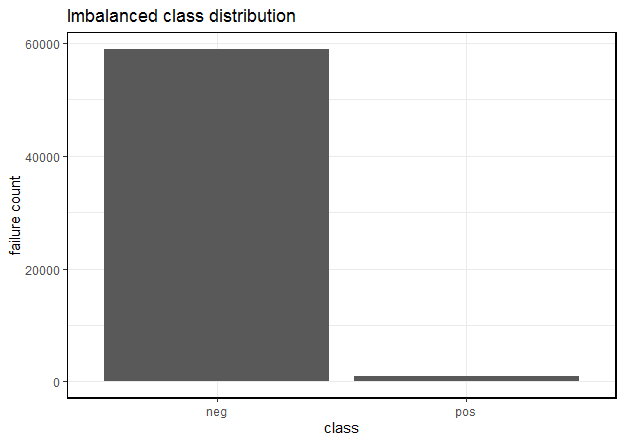
Figure 1: Imbalanced class distribution

ii. Dimensionality reduction steps for training data

The training set contained 60,000 observations in 171 variables of which the dependent variable was binary in nature called, “class”. I had to find the variables that accounted for maximum variance. I took the following measures for dimensionality reduction:

a) Check for variables with more than 75% missing data

I found 6 independent variables that satisfied this property. I removed them from subsequent analysis. The count of independent variables decreased to 165.

b) Check for variables with more than 80% zero values

I found 33 independent variables that satisfied this property. I removed them from subsequent analysis. The count of independent variables decreased to 132.

c) Check for variables where standard deviation is zero

I found 1 independent variable that satisfied this property. I removed it from subsequent analysis. The count of independent variables decreased to 131.

d) Check for variables with near zero variance property

I found 10 independent variables that satisfied this property. I removed them from subsequent analysis. The count of independent variables decreased to 121.

e) Missing data detection and treatment

Since all independent variables were continuous in nature, I used median to impute the missing values in them. In Figure 2, I’ve shown the missing data pattern visualization.

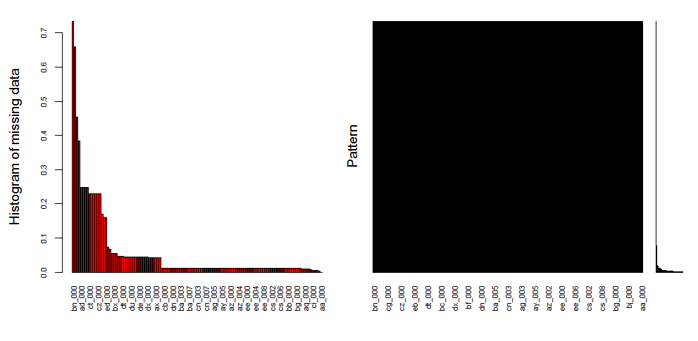
Figure 2: Missing data visualization for training dataset

In Figure 2, the black colored histogram actually shows the missing data pattern. As the number of independent variables was huge, not all of them are shown and hence the color is black.

f) Correlation detection and treatment

I found several continuous variables to be highly correlated. I applied an unsupervised approach, the Principal Component Analysis (PCA) to extract non-correlated variables. PCA also helps in dimensionality reduction and provides variables with maximum variance. In Figure 3, I have shown the important principal components.

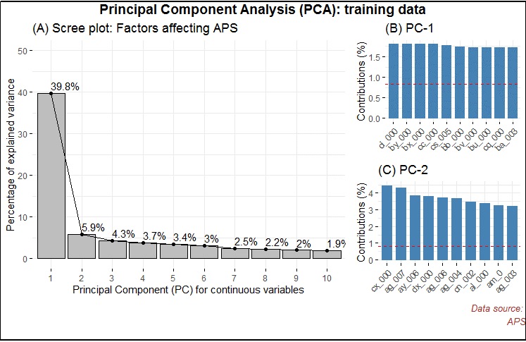
Figure 3: Important principal components for training dataset

C. Predictive modeling

As noted above (see sub-section B-i), this dataset was severely imbalanced. If left untreated, the predictions will be incorrect. I will now show the predictions on the original imbalanced dataset followed by the predictions on the balanced dataset. Thereafter, I’ve provided a discussion on the same.

i. Assumption

In this analysis, my focus is on correctly predicting the positive class, i.e., the trucks with component failures for a specific component of the APS system.

ii. Data splitting

I created a control function based on 3-fold cross validation. Then I split the training set into 70% training and 30% test set. The training dataset contained 42,000 observations in 51 variables. The test set contained 18,000 observations in 51 variables.

iii. Justification on classifier metric choice

Note, I chose Precision Recall Area Under Curve (PR AUC) as a classification metric over Receiver Operating Curve Area Under Curve (ROC AUC).

The key difference is that ROC AUC will be the same no matter what the baseline probability is, but PR AUC may be more useful in practice for needle-in-haystack type problems or problems where the “positive” class is more interesting than the negative class. And this is my fundamental justification to why I chose PR AUC over ROC AUC, because I’m interested in predicting the positive class. This also answers the challenge metric on reducing the type 1 and type II errors.

iv. Predictive modeling on imbalanced training dataset

I chose 3 classifiers namely logistic regression (logreg), linear discriminant analysis (lda) and gradient boosting machine (gbm) algorithms for prediction comparative analysis. I also chose three sampling techniques for data balancing, namely, under sampling, over sampling and synthetic minority over sampling technique (SMOTE). The logistic regression model gave the highest sensitivity.

And in Figure 4, I’ve shown the dot plot which depicts the PR-AUC scores visualization on the imbalanced dataset.

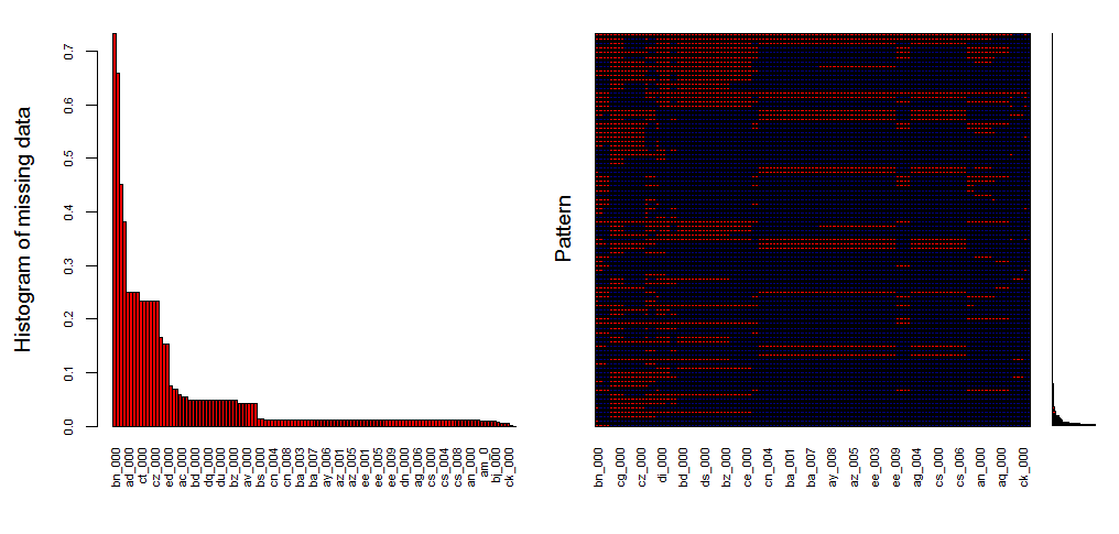
Figure 4: Dot plot on imbalanced training dataset

v. Challenge metric computation on imbalanced training dataset

Challenge metric is the cost metric of misclassification. Where cost 1 = 10 and cost 2 = 500

Total cost = 10 * CM.FP + 500 * CM.FN

Total cost = 1055+500149 = $75, 050

The company will incur $75, 050 in misclassification cost on the imbalanced dataset.

vi. Predictive modelling on balanced training dataset

For data balancing, I chose 3 different methods, namely under-sampling, over-sampling and Synthetic Minority Over Sampling Technique (SMOTE). I found the over sampling technique to be most effective for logistic regression model. So I applied this technique on the balanced training dataset

I’ll now show the predictive modelling on the balanced training dataset. As shown earlier, I split the dataset into 70-30 ratio and applied a 3-fold cross validation. Then, I applied the logistic regression algorithm by up-sampling, down-sampling and synthetic minority over sampling methods shown in Figure 5.

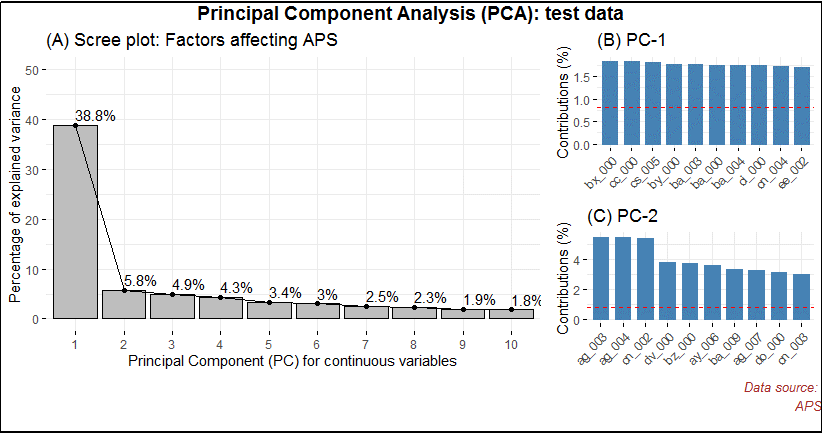
Figure 5: Dot plot on balanced training dataset

vii. Challenge metric computation on balanced training dataset

Challenge metric is the cost metric of misclassification. Where cost 1 = 10 and cost 2 = 500

Over sampling based logistic regression

Total cost = 10 * CM.FP + 500 * CM.FN

Total cost = 10540+50033 = $21,900

The benefit of data balancing is evident. By extracting the independent variables with variance and balancing, I was able to reduce the misclassification cost from the initial $75,050 to $21,900 on the balanced training dataset.

viii. Challenge metric computation on balanced test dataset

Next, I’ll apply the logistic regression over sampled method to the clean test dataset.

Challenge metric is the cost metric of misclassification. Where cost 1 = 10 and cost 2 = 500

Over sampling based logistic regression on test data

Total cost = 10 * CM.FP + 500 * CM.FN

Total cost = 10359+5008 = $7,590

The predicted misclassification cost is found to be $7,590.

Discussion

Oversampling and under sampling can be used to alter the class distribution of the training data and both methods have been used to deal with class imbalance. The reason that altering the class distribution of the training data aids learning with highly-skewed data sets is that it effectively imposes non-uniform misclassification costs. There are known disadvantages associated with the use of sampling to implement cost-sensitive learning. The disadvantage with under sampling is that it discards potentially useful data. The main disadvantage with oversampling, from my perspective, is that by making exact copies of existing examples, it makes over fitting likely. Traditionally, the most frequently used metrics are accuracy and error rate. Considering a basic two-class classification problem, let {p,n} be the true positive and negative class label and {Y,N} be the predicted positive and negative class labels. Then, a representation of classification performance can be formulated by a confusion matrix (contingency table), as illustrated in Table 3. These metrics provide a simple way of describing a classifier’s performance on a given data set. However, they can be deceiving in certain situations and are highly sensitive to changes in data. In the simplest situation, if a given data set includes 5 percent of minority class examples and 95 percent of majority examples, a naive approach of classifying every example to be a majority class example would provide an accuracy of 95 percent. Taken at face value, 95 percent accuracy across the entire data set appears superb; however, on the same token, this description fails to reflect the fact that 0 percent of minority examples are identified. That is to say, the accuracy metric in this case does not provide adequate information on a classifier’s functionality with respect to the type of classification required. Although ROC curves provide powerful methods to visualize performance evaluation, they also have their own limitations. In the case of highly skewed data sets, it is observed that the ROC curve may provide an overly optimistic view of an algorithm’s performance. Under such situations, the PR curves can provide a more informative representation of performance assessment. To see why the PR curve can provide more informative representations of performance assessment under highly imbalanced data, let’s consider a distribution where negative examples significantly exceed the number of positive examples (i.e. N_c>P_c). In this case, if a classifier performance has a large change in the number of false positives, it will not significantly change the FP rate since the denominator N_c is very large. Hence, the ROC graph will fail to capture this phenomenon. The precision metric, on the other hand considers the ratio of TP with respect to TP+FP; hence it can correctly capture the classifiers performance when the number of false positives drastically change. Hence, as evident by this example the PR AUC is an advantageous technique for performance assessment in the presence of highly skewed data. Another shortcoming of ROC curves is that they lack the ability to provide confidence intervals on a classifier’s performance and are unable to infer the statistical significance of different classifiers’ performance. They also have difficulties providing insights on a classifier’s performance over varying class probabilities or misclassification costs. In order to provide a more comprehensive evaluation metric to address these issues, cost curves or PR AUC is suggested.

Conclusion

In this dataset, there were several problems notably the major one was the class imbalance issue, which was followed by missing values and other issues that I’ve highlighted in sub-section 3iii. However, the challenge was not the class imbalance issue per se but the choice of an appropriate metric that could correctly answer the assumption I had formulated in sub-section Ci. The tradeoff between PR AUC and AUC is discussed in sub-section 3iii. Furthermore, I was able to reduce the misclassification cost to $7,590 by over sampling the data.

Appendix A

Explanation of statistical terms used in this study

• Variable: is any characteristic, number or quantity that is measurable. Example, age, sex, income are variables.
• Continuous variable: is a numeric or a quantitative variable. Observations can take any value between a set of real numbers. Example, age, time, distance.
• Independent variable: also known as the predictor variable. It is a variable that is being manipulated in an experiment in order to observe an effect on the dependent variable. Generally in an experiment, the independent variable is the “cause”.
• Dependent variable: also known as the response or outcome variable. It is the variable that is needs to be measured and is affected by the manipulation of independent variables. Generally, in an experiment it is the “effect”.
• Variance: explains the distribution of data, i.e. how far a set of random numbers are spread out from their original values.
• Regression analysis: It is a set of statistical methods used for the estimation of relationships between a dependent variable and one or more independent variables. It can be utilized to assess the strength of the relationship between variables and for modeling the future relationship between them.

Appendix B

The R code for this study can be downloaded from here

comments powered by Disqus