The following data analysis is based on a publicly available dataset hosted at Kaggle. The complete code is located on my github

EXPLORATORY DATA ANALYSIS

• The dataset is a single csv file. It has a shape of 42,542 observations in 144 variables.
  • The response or dependent variable is “loan_status” and is categorical in nature.
• Off the 144 variables, majority of them (~110) are continuous in nature and rest are categorical data types.
• All 144 variables have missing values. - Variables with 80% missing data were removed. The dataset size reduced to 54 variables.
• Correlation treatment helped reduce dataset size to 45 variables. Turns out, independent variables such as funded amount, funded amount inv, installment, total payment, total payment inv, total rec prncp, total rec int, collection recovery fee and pub rec bankruptcies are strongly correlated (>=80%) with the dependent variable.
• By this stage, the dataset shape is 42,542 observations in 45 variables (25 continuous, 3 datetime, and 17 categorical).
• The dependent variable has 4 factor levels. I recoded the 4 factor levels to 2 as asked by the assignment.
  • 34116 observations for loans that were fully paid
  • 8426 observations for loans that were charged off
• The dependent variable was label encoded to make it suitable for model building. As earlier stated, it’s now a binary categorical variable with two levels. Label 1 refers to Fully Paid and Label 0 refers to Charged Off.
• It should be noted, the dependent variable is imbalanced in nature. This means, data balancing method need to be applied for building a robust model.

VISUALS

• A histogram comparing the annual income of applicants from the states of West Virginia (WV) and New Mexico (NM). Is there any relationship here?

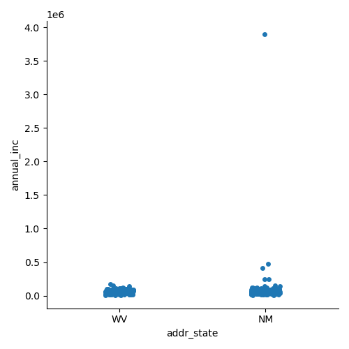
Fig-1: Average annual income of applicants from WV and NM

• The top Top 3 states with highest number of loan defaults are California (CA), New York (NY)and Texas (TX).

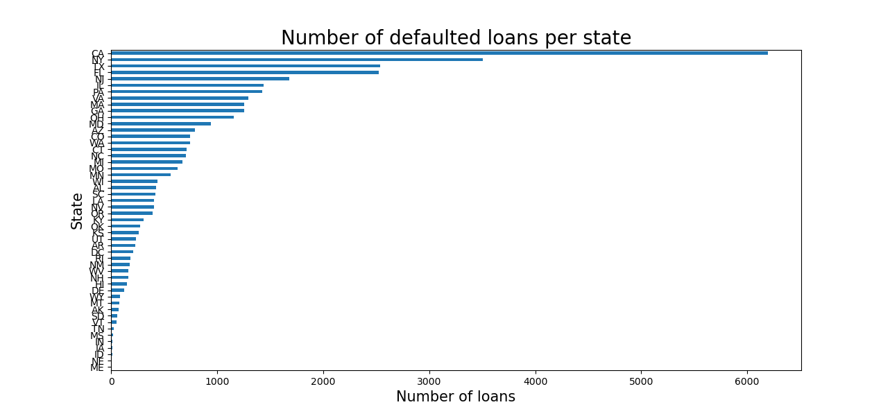
Fig-2: Top 3 states with highest loan defaults

DATA SAMPLING

• To build a classifier model, I took following steps,
  • Data shape at this stage was (42542, 45).
  • Took a 0.05% random sample of the dataset for further analysis.
  • Data shape of sample size was (2127, 45).
  • The reason I took a sample of the original dataset was the presence of several categorical variables with factor levels greater than 5. Label encoding such categorical variables yielded meaningless information in model building and one-hot encoding blew up the dataset size to more than 3GB!
  • Did label encoding for categorical variables with factor levels less than or equal to 2 (term, pymnt_plan, initial_list_status, application_type, hardship_flag, debt_settlement_flag, target).
  • Did one-hot encoding for rest of categorical variables with factor levels greater than 2. Dataset shape becomes (2127, 6965)

MODEL BUILDING

• Null Hypothesis: From Fig-1, its apparent there is no relationship between the average annual income of applicants from WV and NM. To verify this claim further, a significance test is conducted using the ttest_1samp() function from the scipy.stats library.
• Used label encoded data.
• Performed a stratified random sampling to split the dataset into 80% train and 20% test parts (in code, see lines 124 to line 154).
  • Chose logistic regression algorithm
• Building a classification model on imbalanced dependent variable
  • F1 score for loan status with value Charged Off (0) is 90%
  • F1 score for loan status with value Fully Paid (1) is 98%
• Applied synthetic minority over sampling (SMOTE) method for data balancing
  • F1 score for loan status with value Charged Off (0) is 99%
  • F1 score for loan status with value Fully Paid (1) is 100%

Model Summary statistics as follows;

Imbalanced data classification

          precision    recall  f1-score   support
       0       1.00      0.74      0.85        68
       1       0.95      1.00      0.98       358

    accuracy                        0.96       426
   macro avg       0.98      0.87   0.91       426
weighted avg       0.96      0.96   0.96       426

Resampled data shape:  (2856, 6975)
Balanced target
0    1428
1    1428
Name: target, dtype: int64

Balanced data using SMOTE

       precision    recall  f1-score   support

       0       0.98      0.90      0.94        68
       1       0.98      1.00      0.99       358

accuracy                                0.98       426
macro avg       	0.98      0.95      0.96       426
weighted avg        0.98      0.98      0.98       426

End notes

To develop a strategy for risk averse customers, the following points may be considered;

• We should target semi-urban or rural locations. Reason, such areas are replete with middle-economic class and/or lower economic class groups of people. In such sections of society, the penetration of information on Peer to Peer (P2P) lending is low. Our priority should be to educate such masses of people on the benefits and pitfalls of P2P lending as compared to other lending methods.
• Next, such customers can be educated about the Mutual Fund (MF) investment options, in particular the debt MF growth option. This strategy may help to maintain low default rates because the debt MF expense ratio charged by MF companies are comparatively less as compared to equity MF expense ratios.