Introduction
Historically there have been several instance of air plane crashes. This study is an attempt to explore the possible causes of such air crashes, and to determine if air travel is a safe option.
Objective
The objective of this study are two fold, namely;
a. To perform an Exploratory Data Analysis (EDA) to determine the common cause/reason of airplane crash, countries with maximum/minimum airplane crashes, fatalities vs survived ratio and any other interesting trend.
b. To develop a Predictive Model (PM) to determine the following;
- Is traveling by air a safe option?
- In particular analyze the historical data to determine the accuracy of air crash survival.
Data Analysis
A systematic data analysis was undertaken to answer the objectives.
A. Data source
- For this analysis, I have used two data sources. The primary data source was Kaggle and the secondary source was
www.planecrashinfo.com - The dataset hosted on Kaggle was from 1908 till 2009.
- The secondary data source was required because I needed plane crash data from 2010 until 2020. This would help in both EDA and PM.
- So for this analysis, I wrote a custom scrapper to extract the air crash data from
www.planecrashinfo.com
B. Exploratory Data Analysis
Both datasets were dirty. Several data management tasks were carried out to clean the data. As per a researcher Wickham, H. (2014), tidy data is a dataset where each variable is a column and each observation (or case) is a row.
1. Data management decisions
- The Kaggle dataset consisted of 5,268 observations in 13 variables. It had 10,198 missing values
- The external dataset consisted of 237 observation in 13 variables.
- The missing values in external dataset were coded as “?”. These were re-coded to NA. There were 222 missing values.
- The Kaggle dataset and the external data were then merged into a composite dataframe, hereafter referred to as
df. - The
dfconsisted of 5,505 observations in 13 variables. - The range of aircraft crash years was from 1908 till 2020.
ii. Feature engineering
The variable summary contained free form text related to plane crash details. It contained important information. But it needed cleaning. So I created some derived variables like crash_reason, crash_date, crash_month, crash_year, crash_hour, crash_minute, crash_second, crash_area, crash_country, crash_route_start, crash_route_mid, crash_route_end, crash_operator_type, survived, alive_dead_ratio.
C. Data Visualization
As the common adage goes, “a picture is worth a thousand words”. Once the data was cleaned and composed in a tidy format, it was ready for visualizations. Data visualization helps in determining possible relationship between variables. In Fig-1 & Fig-2, I show the common reasons for air crash sorted by descriptions and words. In particular, air crash during take offs are maximum, see Fig-1.
i. Visualizing the common reasons attributed to air plane crash
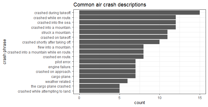
Fig-1: Common air crash descriptions
ii. Visualizing the common words used for air plane crash
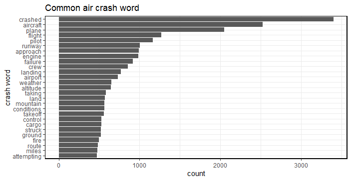
Fig-2: Common air crash words
iii. Visualizing the crashed flight operators
A majority of the flight operators are US-military, AirForce, Aeroflot, Air France and Luftansa, as seen from Fig-3.
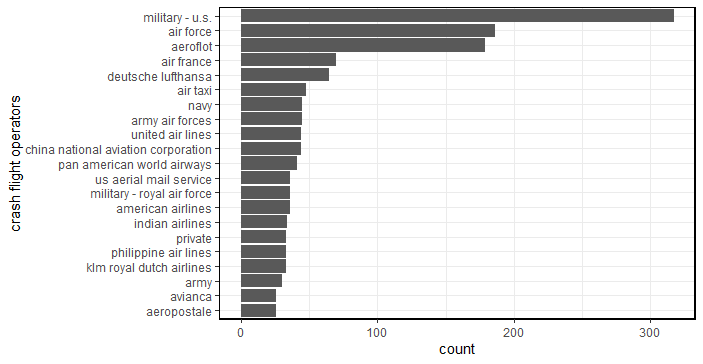
Fig-3: Air crash flight operators
The peak of air crash survivors was in year 2000, see Fig-4. Probably the reason could be because of better aircraft’s compared to yesteryear’s.
iv. Visualizing the air crash survivors
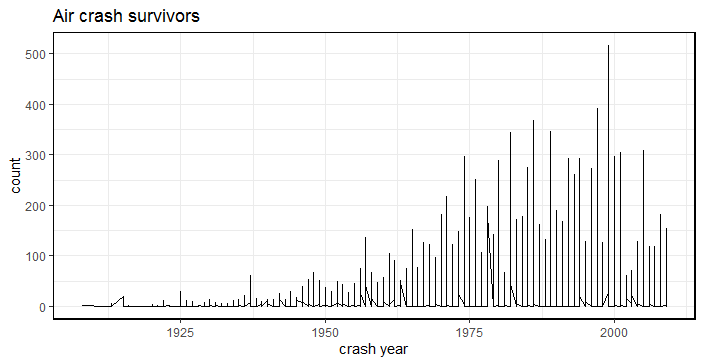
Fig-4: Air crash survivors by year
It was found that there were more civilian air crashes as compared to military crashes. Moreover, 3,198 fatalities are observed in air crashes since 1908, including both civilian and military air crashes. So, I took a subset of the civilian air crashes data and plotted it. I present them below in the form of some hypothesis.
v. Visualizing the civilian air crash fatalities
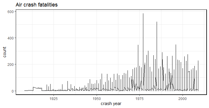
Fig-5: Civilian air crash survivors by year
-
The peak of air crashes lay between the years 1970-1980s.
-
Off these 58 aircraft’s crashed in Alaska, followed by 45 in Russia, 32 and 30 in Colombia and California respectively.
-
I then filtered data for crash year after year 2010 and found that Russia recorded maximum civilian fatalities in year 2011 (dead=5), followed by Indonesia in year 2015 (dead=4) and Russia in year 2012 (dead=4). See Fig-5.
vi. Is there a relationship between civilian air crash year and crash reason
I plotted this relationship and found the following:
- There were 4,692 civilian air crashes since 1908 and 813 military induced air crashes. See Fig-6.
- Off these 4,692 civilian air crashes, 644 occurred after year 2000.
- Off the 644 civil air crashes, 301 were technical failures, 86 by natural cause, 52 crashed in mountains and 7 were shot down by military. There are 198 uncategorized crashes.
- The civilian aircrafts shot down by military crashed in countries like Congo (year 2003), Iran (year 2020), Laos (year 2014), Kedarnath, India (year 2013), Rapua (year 2016), Russia (year 2001) and Zabul province (year 2010).
- Majority of civil air crashes were due to technical failure. At least 4 aircrafts crashed in Russia in 2011 because of technical failure. This was followed by Sudan, where 3 planes were lost in 2008 because of technical failure. Since the year 2010, there were 20 civilian aircraft crashes for Russia, 10 for Nepal, followed by Congo and Indonesia at 9 each.
- The median for military action related air crash was around year 1951
- The median for mountain and natural caused crashes was around year 1976
- The median for technical failure related crashes was around 1977.
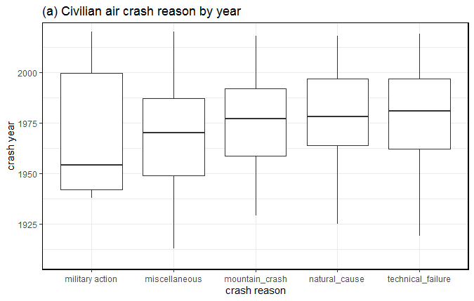
Fig-6: Reasons for civilian air crashes sorted by year
vii. Is there a relationship between civilian air crash month and crash reason
I plotted this relationship and found the following:
- A majority of air crashes took place around the month of July. These crashes were related to mountain, natural, miscellaneous and natural reasons. See Fig-7.
- Russia tops this list with 7 air crafts crashing in July month because of technical failure. Off these 7 air crafts, 4 were of Antonov An series.
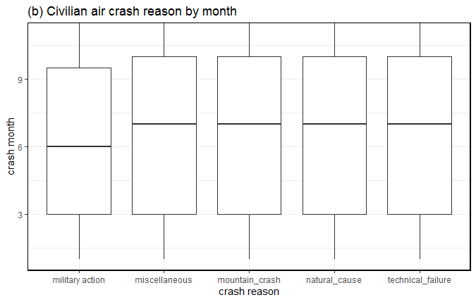
Fig-7: Reasons for civilian air crashes sorted by month
viii. Is there a relationship between civilian air crash fatalities and crash reason
Although the median for civilian air crash fatalities normally centered around 1-5 people, but there were several outlier values too. For instance in one military action induced civil aircraft crash took the life of all 290 people aboard. This incident occurred in 1988 at 10:55pm over the Persian Gulf, near Bandar Abbas in Iran. The Airbus A300B2-203 bearing registration number EPIBU was shot down by an US Navy vessel USS Vincennes by a SAM (surface to air) missile. See Fig-8.
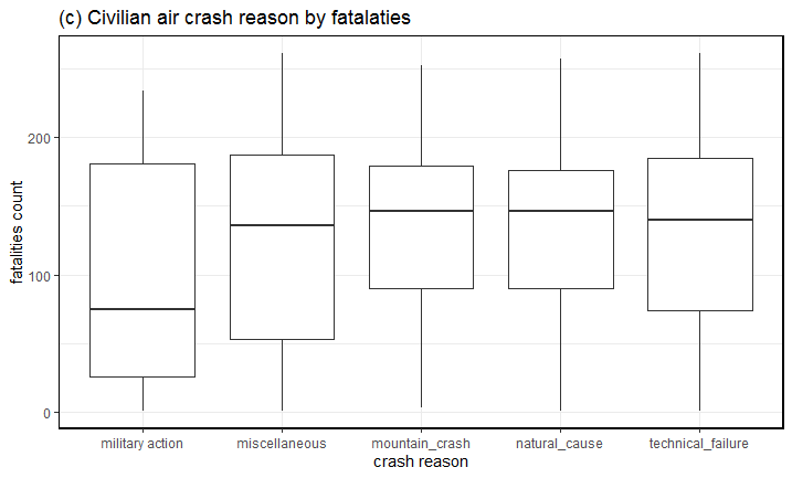
Fig-8: Reasons for civilian air crashes sorted by fatalities
D. Data sub setting
Looking at the data distribution, I found maximum observation were related to civilian aircraft crashes (n=4692) while the observations for military aircraft crashes were less (n=813). Furthermore, I subset the civilian air craft crashes since the year 2010. The reasoning is, to answer the first objective, “is travelling by air a safe option”, I needed to analyze the data for the last one decade. The data dimension for civilian air craft crash since year 2010 was 205 observations in 24 variables (includes both original & derived variables).
E. Detecting Near Zero Variance (NZV)
NZV is a property wherein a given variable has almost zero trend, i.e. all its values are identical. I found two such variables in civilian aircraft crashes. They were, “ground” & “crash operator type”. I removed them from further analysis. I also removed the summary variable. At this stage, the data dimension for civilian air craft crash since year 2010, was 205 observations in 21 variables (includes both original & derived variables)
F. Missing data analysis
There are two types of missing data:
-
Missing Completely At Random (MCAR): is a desirable scenario
-
Missing Not At Random: is a serious issue and it would be best to check the data gathering process.
For this analysis, I’m assuming the data is MCAR. Usually a safe minimal threshold is 5% of the total for a dataset. For a given variable, if the data is missing for more than 5% then it’s safe to leave that variable out of analysis. Basis of this assumption, I found the following variables, Crash_hour, Crash_minute, Flight, Crash_route_start, Crash_route_mid, Crash_route_end, Fuselage_number, with more than 5% missing data.
It should be noted that for civilian aircraft crashes since 1908, in all there were 16051 observations with missing data. Furthermore, for civilian aircraft crashes since 2010, there were 370 missing values. Since the sample size was small (n=205), I imputed the missing values as Zero.
G. Correlation detection
In building a predictive model, it’s always advisable to account for correlation. It is a statistical term that measures the degree of linear dependency between variables. So variables that are highly correlated to each other are deemed to be non-contributors to a given predictive model. In Fig 9, I show the correlation plot for continuous variables. For instance, the variable aboard and fatalities have a strong negative correlation.
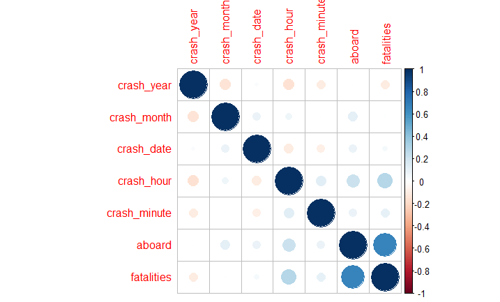
Fig-9: Correlation detection for continuous variables
i. Correlation treatment
To treat the correlation, I have applied an unsupervised dimensionality reduction and feature selection approach called the Principal Component Analysis (PCA) for continuous variables, and the Multiple Correspondence Analysis (MCA) for the categorical variables. In Fig-10, I have shown relevant principal components (PCs). Notice the red horizontal line in Fig 10 (B). This red line indicates the cut-off point. Therefore the continuous variables namely, “aboard, fatalities, crash minute, crash month, crash date, crash year” are deemed relevant for further analysis.
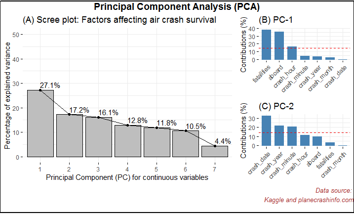
Fig-10: Principal Component Analysis for dimensionality reduction & feature selection
Next, In Fig-11, I have shown the MCA for categorical variables. Notice the red horizontal line in Fig-11 (B). This red line indicates the cut-off point. As we can see from this plot that none off the categorical variables are deemed relevant for further analysis.
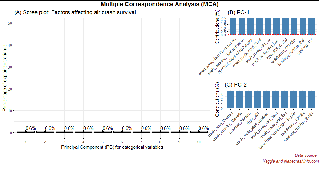
Fig-11: Multiple Correspondence Analysis for dimensionality reduction & feature selection
By this stage, the data dimension for air craft crashes since 2010 was reduced to 205 observation in 7 variables.
H. Predictive analytics
The derived variable survived was continuous in nature. For a classification task, I coerced it into categorical with two levels. If there were 0 survivors, then I coded it as “dead” and if there were more than 1 survivor, it was coded as alive and saved it as a variable called crash survivor.
I found that in 205 complete clean observations, the proportion of dead was 63% and that of alive was 37%. This indicated that the outcome/dependent variable crash survivor was imbalanced. If this anomaly is left untreated, then any model based on this variable will give erroneous results. An imbalanced dataset refers to the disparity encountered in the dependent (response) variable.
Therefore, an imbalanced classification problem is one in which the dependent variable has imbalanced proportion of classes. In other words, a data set that exhibits an unequal distribution between its classes is considered to be imbalanced. I split the clean dataset into a 70/30 % split by 10-fold cross validation. The training set contained 145 observations in 7 variables. The test set contained 60 observations in 7 variables. The 7 independent variables are, crash year, crash month, crash date, crash minute, aboard, fatalities and crash survivor.
i. Methods to deal with imbalanced classification
- Under Sampling
With under-sampling, we randomly select a subset of samples from the class with more instances to match the number of samples coming from each class. The main disadvantage of under-sampling is that we lose potentially relevant information from the left-out samples.
- Over Sampling
With oversampling, we randomly duplicate samples from the class with fewer instances or we generate additional instances based on the data that we have, so as to match the number of samples in each class. While we avoid losing information with this approach, we also run the risk of over fitting our model as we are more likely to get the same samples in the training and in the test data, i.e. the test data is no longer independent from training data. This would lead to an overestimation of our model’s performance and generalization.
- ROSE and SMOTE
Besides over- and under-sampling, there are hybrid methods that combine under-sampling with the generation of additional data. Two of the most popular are ROSE and SMOTE.
The ideal solution is, we should not simply perform over- or under-sampling on our training data and then run the model. We need to account for cross-validation and perform over or under-sampling on each fold independently to get an honest estimate of model performance.
ii. Prediction on imbalanced dataset
To test the accuracy of air crash survivors, I applied three classification algorithms namely Classification and Regression Trees (CART), K-Nearest Neighbors (KNN) and Logistic Regression (GLM) to the clean imbalanced dataset. The CART and GLM model give 100% accuracy. See Fig-12.
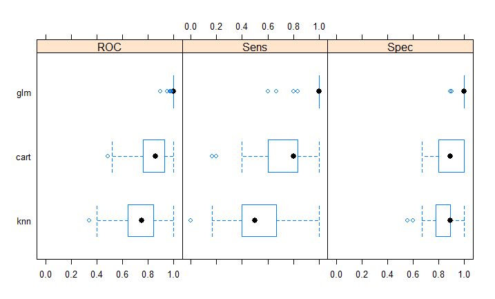
Fig-12: Accuracy plot of predictive models on imbalanced data
I have shown below the predictive modelling results on imbalanced dataset.
Call:
summary.resamples(object = models)

Models: cart, knn, glm
Number of resamples: 100

ROC
  Min.   1st Qu.Median  Mean   3rd Qu. Max. NA's
cart 0.4907407 0.7666667 0.8605556 0.8390667 0.933796310
knn  0.3444444 0.6472222 0.7527778 0.7460315 0.845833310
glm  0.9000000 1.0000000 1.0000000 0.9977593 1.000000010

Sens
  Min. 1st Qu. Median  Mean   3rd Qu. Max. NA's
cart 0.1666667 0.60.8 0.7310000 0.833333310
knn  0.0000000 0.40.5 0.5406667 0.666666710
glm  0.6000000 1.01.0 0.9723333 1.000000010

Spec
  Min.   1st Qu.Median  Mean   3rd Qu. Max. NA's
cart 0.6666667 0.8000000 0.8888889 0.8846667 1.000000010
knn  0.5555556 0.7777778 0.8888889 0.8461111 0.888888910
glm  0.8888889 1.0000000 1.0000000 0.9801111 1.000000010
Confusion Matrix and Statistics

  Reference
Prediction alive dead
 alive220
 dead  0   38

   Accuracy : 1
 95% CI : (0.9404, 1)
No Information Rate : 0.6333
P-Value [Acc NIR] : 1.253e-12

  Kappa : 1
 Mcnemar's Test P-Value : NA

Sensitivity : 1.0000
Specificity : 1.0000
 Pos Pred Value : 1.0000
 Neg Pred Value : 1.0000
 Prevalence : 0.3667
 Detection Rate : 0.3667
   Detection Prevalence : 0.3667
  Balanced Accuracy : 1.0000

   'Positive' Class : alive
From the result above, its evident the sensitivity of CART and GLM model is maximum.
iii. Prediction on balanced dataset
I balanced the dataset by applying under, over sampling method as well as the ROSE method. From the results shown in above, I picked the logistic regression model to train on the balanced data. As we can see now, the sensitivity for over and under-sampling is maximum when applied the logistic regression algorithm. So I chose, under sampling for testing the model. See Fig-13 and the confusion matrix results are shown below.
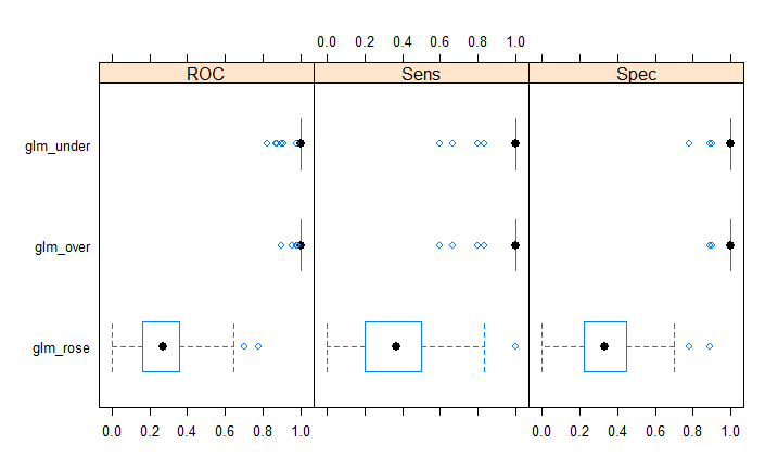
Fig-13: Accuracy plot of predictive models on balanced data
After balancing the data and reapplying a logistic regression algorithm, the accuracy to predict the air crash survivor accuracy reduced to 98%, as shown in confusion matrix below.
Call:
summary.resamples(object = models)

Models: glm_under, glm_over, glm_rose
Number of resamples: 100

ROC
   Min.   1st Qu.Median  Mean   3rd Qu.  Max.
glm_under 0.8240741 1.0000000 1.0000000 0.9920185 1.0000000 1.0000000
glm_over  0.9000000 1.0000000 1.0000000 0.9977593 1.0000000 1.0000000
glm_rose  0.0000000 0.1638889 0.2722222 0.2787333 0.3555556 0.7777778
  NA's
glm_under0
glm_over 0
glm_rose 0

Sens
  Min. 1st Qu.Median  Mean 3rd Qu. Max. NA's
glm_under  0.6 1.0 1.0000000 0.9746667 1.010
glm_over   0.6 1.0 1.0000000 0.9723333 1.010
glm_rose   0.0 0.2 0.3666667 0.3533333 0.510

Spec
   Min.   1st Qu.Median  Mean   3rd Qu.  Max.
glm_under 0.7777778 1.0000000 1.0000000 0.9745556 1.0000000 1.0000000
glm_over  0.8888889 1.0000000 1.0000000 0.9801111 1.0000000 1.0000000
glm_rose  0.0000000 0.2222222 0.3333333 0.3538889 0.4444444 0.8888889
  NA's
glm_under0
glm_over 0
glm_rose 0
 Confusion Matrix and Statistics

  Reference
Prediction alive dead
 alive221
 dead  0   37

   Accuracy : 0.9833
 95% CI : (0.9106, 0.9996)
No Information Rate : 0.6333
P-Value [Acc > NIR] : 4.478e-11

  Kappa : 0.9645
 Mcnemar's Test P-Value : 1

Sensitivity : 1.0000
Specificity : 0.9737
 Pos Pred Value : 0.9565
 Neg Pred Value : 1.0000
 Prevalence : 0.3667
 Detection Rate : 0.3667
   Detection Prevalence : 0.3833
  Balanced Accuracy : 0.9868

   'Positive' Class : alive
iv. Results interpretation
In answering the second objective of this analysis, it’s been found that the logistic regression model gives 98% accuracy in determining the accuracy of an air crash survival. This explains the need for balancing the dataset before modeling.
I. Limitations
Perhaps, one of the challenges on working on this dataset was the higher number of categorical variables. And each such variable having more than 10 distinct levels. Decomposing them into a smaller number of meaningful levels would require help from a subject matter expert. Besides this, the dataset contained a huge number of missing values in categorical variables. Imputing them would be bottleneck to the primary memory. I replaced the missing values with Zero.
J. Discussion
There can be an argument on the necessity of data balancing. For instance, in this analysis I have shown that imbalanced data give 100% accuracy, in contrast the balanced data accuracy reduces to 98%. The reasoning here is, balanced or imbalanced data is dependent on distribution of data points. By balancing the data, the analyst is absolutely certain about the robustness of the model, which would not be possible with an imbalanced dataset.
Traveling by air is certainly a safe option in present times. I have proved this claim by conducting a systematic rigorous data analysis. Moreover, the logistic regression model trained on balanced under-sampled data yield the maximum sensitivity.
K. Conclusion and Future Work
In this study, I have analyzed the last 101 years data on air craft crashes. I have shown in my detailed analysis that given certain factors like crash year, crash month, crash date, crash minute, aboard, fatalities and survived, it’s possible to predict the accuracy of air crash survivors. I have tested several hypothesis in this work, see section C. It would be interesting to see trends between aircraft type and air crash fatalities which I leave as a future work.
Reference
Wickham, H. (2014). Tidy data. Journal of Statistical Software, 59(10), 1-23.
Appendix A
Explanation of statistical terms used in this study
- Variable: is any characteristic, number or quantity that is measurable. Example, age, sex, income are variables.
- Continuous variable: is a numeric or a quantitative variable. Observations can take any value between a set of real numbers. Example, age, time, distance.
- Categorical variable: describes quality or characteristic of a data unit. Typically it contains text values. They are qualitative variables.
- Categorical-nominal: is a categorical variable where the observation can take a value that cannot be organized into a logical sequence. Example, religion, product brand.
- Independent variable: also known as the predictor variable. It is a variable that is being manipulated in an experiment in order to observe an effect on the dependent variable. Generally in an experiment, the independent variable is the “cause”.
- Dependent variable: also known as the response or outcome variable. It is the variable that is needs to be measured and is affected by the manipulation of independent variables. Generally, in an experiment it is the “effect”.
- Variance: explains the distribution of data, i.e. how far a set of random numbers are spread out from their original values.
- Sensitivity: is the ability of a test to correctly identify, the occurrence of a value in the dependent or the response variable. Also known as the true positive rate.
- Specificity: is the ability of a test to correctly identify, the non-occurrence of a value in the dependent or the response variable. Also known as the true negative rate.
- Cohen’s Kappa: is a statistic to measure the inter-rate reliability of a categorical variable. It ranges from -1 to +1.
Appendix B
The R code for this study can be downloaded from here
comments powered by Disqus